Will MLX replace PyTorch? Exploring MLX (Part-1)
Apple has just dropped a bombshell in the world of machine learning by releasing its very own open-source framework, MLX. Yep, that’s right Apple and open-source in the same sentence! 🤩. So, naturally, I did what any curious mind would do: I fired up my livestream and embarked on an epic journey to uncover the ins and outs of MLX.
I wanted to dive deep into MLX's workflow and put it to the test by building a CNN-based MNIST Classifier. But wait, there's more! I didn't stop there—I also decided to throw PyTorch into the mix for a 1v1 showdown. After all, PyTorch is one of the heavyweights in the world of deep learning frameworks, so what better way to gauge MLX's performance, right? So, what did I compare, you ask? Well, I focused on analyzing the training time and accuracy. And let me tell you, the results were mind-blowing! If you're anything like me and love getting hands-on with the development process, then you're in luck! You can catch all the action on my YouTube channel.
But enough chit-chat! Let's cut to the chase and dive straight into the world of Apple's very own deep learning framework, MLX.
All the code mentioned in this blog is available on GitHub.
Coding Part
MLX's documentation proved to be an invaluable resource throughout our coding journey, guiding us every step of the way without the need to seek additional references. Their comprehensive documentation not only provided clear explanations but also included practical examples, like the MNIST classifier, which served as a solid foundation for our project. Although the example provided by MLX utilized feed-forward layers, we were able to leverage their mnist.py file to seamlessly load the MNIST dataset into our workflow. Drawing from our familiarity with PyTorch, the model creation and training process felt like second nature, with no major hurdles encountered along the way. Take a peek at the code snippet below, showcasing our model class. At first glance, it's strikingly reminiscent of code written in PyTorch, with just a few minor tweaks to adapt to MLX's syntax and conventions:
# Model Definition Syntax in MLX
class CNN(nn.Module):
    def __init__(self, output_dim):
        super().__init__()
        self.layers = [nn.Conv2d(1, 32, kernel_size = 3), nn.Linear(26 * 26 * 32, 256), nn.Linear(256, output_dim)]

    def __call__(self, x):
        for i in range(len(self.layers[:-2])):
            l = self.layers[i]
            x = mx.maximum(l(x), 0.0) # relu activation

        x = x.reshape(x.shape[0], -1)
        x  = mx.maximum(self.layers[-2](x), 0.0)
        return self.layers[-1](x)
As you can see, the transition from PyTorch to MLX was smooth sailing, thanks to the intuitive design of MLX and our prior experience with deep learning frameworks.
# Model Definition Syntax in Python
class CNN(nn.Module):
    def __init__(self, output_dim):
        super().__init__()
        self.l1 = nn.Conv2d(1, 32, kernel_size = 3)
        self.l2 = nn.Linear(26 * 26 * 32, 256)
        self.l3 = nn.Linear(256, output_dim)

    def forward(self, x):
        x = F.relu(self.l1(x))
        x = x.view(x.shape[0], -1)
        x  = F.relu(self.l2(x))
        return self.l3(x)
At the time of the livestream, MLX lacked implementations for AvgPool2D and MaxPool2D layers. To overcome this obstacle, I set out to design custom layers for the same. However, to my dismay, I discovered that my model hit a roadblock—it stopped learning when utilizing custom AvgPool2D layers. It turned out that MLX's AutoGrad function struggled to backpropagate through these custom layers, hindering the learning process. As a result, I had to delay my plans for integrating custom layers into MLX but rest assured, it's something I'm eager to tackle in future episodes of the series.
Now, let's talk about the training loop. While it bears a striking resemblance to the training loop in PyTorch, there are some subtle differences, particularly in how MLX handles the loss function. In MLX, rather than using the loss function directly, it is passed to a value_and_grad function provided by mlx alongside our model. During the training, this function is used to compute both the loss and gradients for model parameters. These gradients are subsequently passed to the optimizer's update function along with our model, allowing the optimizer to update the model's parameters based on the provided gradients.
Despite these nuances, the essence of the training loop remains similar to other frameworks: iteratively adjusting the model's parameters to minimize the loss and improve performance.
# Defining the training loop for our model in MLX
model = CNN(10)
mx.eval(model.parameters())

loss_and_grad_fn = nn.value_and_grad(model, loss_fn)
optimizer = optim.SGD(learning_rate = lr)
accuracies = []

start_time = time.time()
for e in range(num_epochs):
     for X, y in batch_iterate(batch_size, train_images, train_labels):
          loss, grads = loss_and_grad_fn(model, X, y)

          optimizer.update(model, grads)

          mx.eval(model.parameters(), optimizer.state)
     accuracy = eval_fn(model, test_images, test_labels)
     accuracies.append(accuracy.item())
     print(f"Epoch {e}: Test accuracy {accuracy.item():.3f}")
end_time = time.time()
While I was replicating the MLX model in PyTorch, I stumbled upon a fascinating discovery that left me scratching my head. Initially, I attempted to normalize the input images by simply dividing them by 255.0—a seemingly straightforward approach. However, to my surprise, my PyTorch model was not learning at all with this naive normalization method.
After some trial and error, I decided to enlist the help of PyTorch's Normalize function instead of my approach to normalization, and voila! Suddenly, everything clicked into place, and my model began to learn as expected. But why did this happen? Why did my naive normalization fail to yield results? On the surface, my normalization should have constrained the input values to a range between 0 and 1, which theoretically should have worked just fine. But alas, the mystery remains unsolved.
I share this experience with you not only to shed light on my journey but also to offer a word of caution.
So, if you find yourself facing a similar challenge in your deep learning endeavours, fear not! Take a leaf out of my book, and don't hesitate to explore alternative approaches. And if you happen to crack the code behind this mystery, be sure to drop a comment on the YouTube video or contact me via any social media handle—I'd love to hear your insights!
Results Part
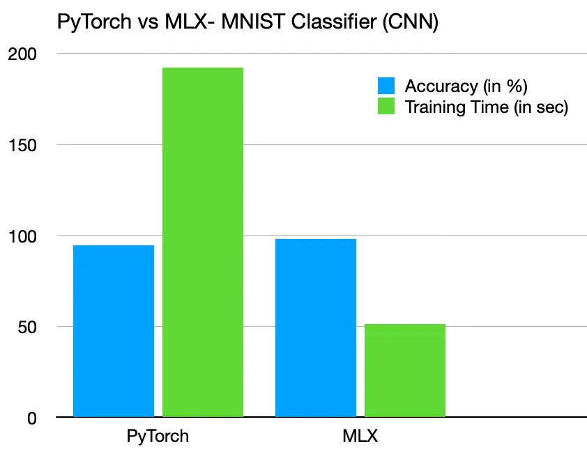
It's truly remarkable how MLX manages to deliver a 4x training speed boost compared to PyTorch. But here's the twist: despite wielding identical hyperparameters, models, and optimizers, MLX consistently falls short in the accuracy department when pitted against PyTorch. Now, isn't that a head-scratcher?
| FrameWork | Avg. Training Time | Avg. Accuracy |
|---|---|---|
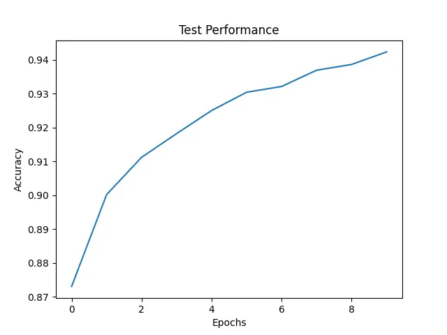
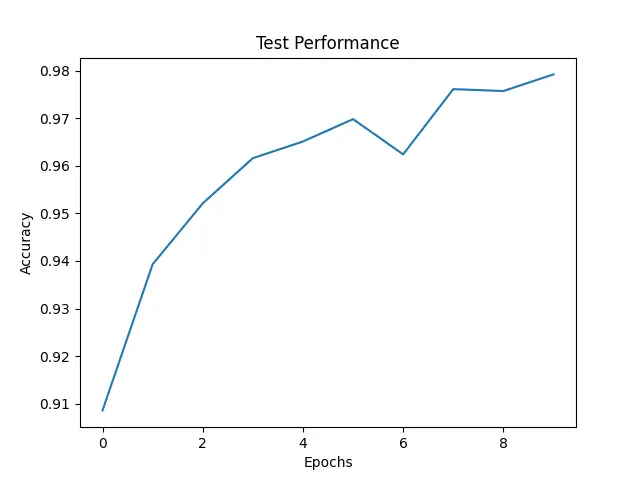
| MLX | 51.352 sec | 0.945 |
| PyTorch | 192.332 sec | 0.978 |
While this discrepancy in accuracy has left me scratching my head, I'm determined to get to the bottom of it in the upcoming episodes of our journey. Despite its accuracy woes, MLX's training process seems impressively stable. Perhaps with a slight tweak to our strategy—increasing the number of epochs and extending the training time ever so slightly—we may just be able to bridge the gap and achieve comparable results to PyTorch in a fraction of the time. But that is not the goal of this episode, here our target was to compare the performance of MLX and PyTorch when provided with similar working environments on a M1 Mac.
So, buckle up and stay tuned for the next thrilling instalment of our journey, where we'll dive deeper into the mysteries of MLX and uncover the secrets to unlocking its full potential.